Getting Started
This guide will familiarise your with the concepts necessary to run analyses in SMCSMC and take you through the basic aspects of an analysis using toy data. You may also be interested in one of several examples using real and simulated data in the Tutorials section.
Note
This tutorial is intended to be run on a personal computer, and values have been scaled accordingly. For analysis on real data, we expect that a user will have access to a compute cluster, and we provide guidance about setting up smcsmc to function with common architechtures in Clustering Computing.
Basic Concepts
SMCSMC is a particle filter, which means that a given number of particles are simulated, evaluated for an approximate likelihood, and resampled until demographic parameters have converged. Many of the options relate to the behaviour of this particle filter, and the remainder deal with the demographic model that you wish to infer. SMCSMC can infer complex demographic models involving several populations, though you should be weary of overspecifying your model. Run time increases drastically with the number of parameters needed to specify the model.
Input Format
Suppose we have the following data, saved into a file named toy.seg. You can also download it here.
| segment start | segment length | invariant | break | chr | genotype |
|---|---|---|---|---|---|
| 1 | 521 | T | F | 1 | 01.0 |
| 522 | 2721 | T | F | 1 | 0111 |
| 3243 | 1758 | T | F | 1 | 10// |
| 5001 | 1296 | T | F | 1 | 0000 |
| 6297 | 1 | T | F | 1 | …. |
| 6298 | 4669 | T | F | 1 | 0110 |
| 10967 | 880 | T | T | 1 | 0100 |
| 1 | 708 | T | F | 2 | 1010 |
This gives the state of four haplotypes along the sequence, indicating segment starts and their lengths. If a segment is the last in a block before coordinates reset (i.e. when including multiple chromosomes in a single seg file, it is called a genetic break. Genotypes in terms of either major/minor or ancestral/derived are given for each haplotype. Missing data is coded with a period (.) whilst unphased variants are given with a forward slash (/).
Note
This data format is similar to the input for msmc however, in the second column we require the length from the current segment to the next, rather than the number of called sites from the previous segment to the current one.
Segment files are specified by the seg flag, or if more than one are used, by the segs flag. Globs are encouraged for readability. In the case of multiple files, genetic breaks are inferred from the beginnings and ends of files. Additionally, we tell smcsmc the number of samples we expect with nsam, so it knows to check the seg file for formatting issues.
Basic Arguements
In addition to the segment file, we need a few more pieces of information to kick off the particle filter.
Particle Count: We must specify a particle count (Np) or use the default value of 1000. The number of particles refers to the number of individual ARGs which are simulated by SCRM, higher numbers means that the model is more likely to converge on a reasonable answer, but increasing the particle count is computationally expensive. We recommend particle counts between 25 and 50 thousand for analysis. However, for exploratory work, smaller particle counts (a good starting point is 10 thousand) can be used to more effectively use computational resources. In this guide, intended for use on a personal computer, we will use 10 particles.
Number of Iterations: We also explictly define the number of expectation maximization iterations that we want to use (EM). A good place to start is 15 iterations. smcsmc looks for output before starting, so should you be unsatisfied with the convergence after 15 iterations, simply run the exact same program with a higher number of iterations. smcsmc will find the output for the iterations already run and simply continue from where it left off.
Demographic Parameters: Several arguements are good to specify, especially when analysing real data as they help with convergence. Here we will use a mutation rate (mu) of 1.25e-8 and a recombination rate (rho) of 3e-9. We give an effective population size (N0) of 14312, and infer trees back to 4*N0 generations with tmax. We set this to 3.5, which is 1.2 Mya with an N0 of 10000. smcsmc infers demographic parameters as discrete over intervals. We specify 31 intervals evenly spaced on the log scale with P 133 133032 31*1 giving the end times of the first and last epochs in generations, and the pattern for their generation.
We also give the path to the output folder with o.
Running smcsmc
Tip
It is always a good idea to start a new conda environment for a new analysis to ensure that there are no dependecy conflicts, though you can skip this step if you certain that your environment is correctly configured.
conda create --name smcsmc_tutorial
conda activate smcsmc_tutorial
Once smcsmc is installed, we can format the arguements detailed above into a dictionary.
import os

args = {
   'seg':                  'toy.seg',
   'nsam':                 '4',
   'Np':                   '10',
   'EM':                   '1',
   'mu':                   '1.25e-8',
   'rho':                  '3e-9',
   'N0':                   '10000',
   'tmax':                 '3.5',
   'P':                    '133 133032 31*1',
   'no_infer_recomb':      '',
   'smcsmcpath':           os.path.expandvars('${CONDA_PREFIX}/bin/smcsmc'),
   # The minimum segment length is usually best left
   # as the default, however for this tutorial we set it
   # artifically low.
   'minseg':               '10',
   'o':                    'smcsmc_output'
}
We directly use this dictionary with the run_smcsmc command, which takes as its only arguement a dictionary of arguements.
import smcsmc
smcsmc.run_smcsmc(args)
If your installation has been successful, then this will begin the process of parsing the input, merging any given seg files, starting the particle filter, and iterating through the EM steps requested.
Output
If your smcsmc has run correctly, the resulting output directory will look something like this, with a seperate folder for each EM iteration, and a seperate file for each chunk, if this option has been used.
output/
        emiterN/
                chunkN.out
                chunkN.stdout
                chunk.stderr
                chunkfinal.out
        merged.seg
        merged.map
        result.log
        result.out
If you are following this tutorial and are only using a single input seg file, you will not see merged.seg or merged.map as there was no need to generate them. The output for each chunk is given, along with stdout and sterr, and results are aggregated over all chunks each epoch into chunkfinal.out. The final epoch will be post processed into result.out. Output and debugging information along with useful information to help interpret the results of your model are given in result.log.
An example of a results.out file is given here:
Iter  Epoch       Start       End   Type   From     To            Opp          Count           Rate             Ne         ESS  Clump
15      0           0         133   Coal      0     -1      307466.77      18.798649  6.1140424e-05      8177.8955      1.0272     -1
15      0           0         133   Coal      1     -1      324087.66      55.469939  0.00017115721      2921.2909      1.0225     -1
15      1         133       166.2   Coal      0     -1       167571.8      1.0002328  5.9689802e-06      83766.402      1.0791     -1
15      1         133       166.2   Coal      1     -1      174231.23    0.067992116  3.9024069e-07      1281260.5      1.0674     -1
15      2       166.2      207.68   Coal      0     -1      259801.05      40.479172  0.00015580835      3209.0707      1.1686     -1
15      2       166.2      207.68   Coal      1     -1      267803.96  0.00028150086  1.0511452e-09  4.7567166e+08      1.1522     -1
15     -1           0       1e+99  Delay     -1     -1  2.6001037e+09              0              0              0           1     -1
15     -1           0       1e+99   LogL     -1     -1              1      -31005174      -31005174              0           1     -1
15      0           0         133   Migr      0      1       178112.7      7.1251662  4.0003695e-05              0      1.0385     -1
15      0           0         133   Migr      1      0      186343.02  0.00022362676  1.2000812e-09              0      1.0338     -1
15      1         133       166.2   Migr      0      1       87712.37      0.5934193  6.7655144e-06              0      1.0819     -1
15      1         133       166.2   Migr      1      0       91253.03      3.0913275  3.3876437e-05              0      1.0713     -1
15      2       166.2      207.68   Migr      0      1      134755.98      1.0135379  7.5212833e-06              0      1.1711     -1
15      2       166.2      207.68   Migr      1      0      139267.34      6.0189739  4.3218847e-05              0      1.1565     -1
The full interpretation of the output is somewhat involved, and we recommend referring to the supporting publication for a complete explaination of all relevant quantities. However, in brief:
- Iter: The EM iteration to which this file refers. In the case of aggregated files (
chunkfinal.out,result.out), multiple iterations are represented in the same file, and it is often useful either to graph each iteration seperately to show convergence, or to select the last iteration to show the final inference. - Epoch: The discrete piece of time in which rates are assumed to be constant. The pattern which epochs follow is set by the
Pflag. - Start: The beginning of the epoch, in generations.
- End: The end of the poch, in generations.
- Type: Either
Coal(coalescence),Delay,LogL(Log likelihood), orMigr. The important lines for interpreting output are:Coal: This line refers to coalescent events. ForCoalevents, theFromrefers to the population of interest while theTois meaningless. An estimate ofNeis shown only inCoallines.Migr: This line refers to migration events.FromandTorefer to the source and the sink of migration, backwards in time.
- Opp: The possible time where events of this can may happen in this sequence. For recombination inference, this refers to the amount of time multiplied by the amount of sequence.
- Count: The number of events of this type inferred in this epoch.
- Rate: Either the coalescent, recombination, or migration rate. This is equal to the
Countdivided byOpp. Coalescent rates are number of coalescentn events per generation. Migration rates represent proportion migration from the source (From) to the sink (To) backwards in time.
Note
SCRM reports migration rates forwards in time while smcsmc reports it backwards in time.
- Ne: The estimated population size in this epoch. Defined to be
Oppdivded by2*Count. - ESS: Effective sample size, which is an indicator of the diversity of our particles. This is used when deciding to resample, or when to spawn new particles.
- Clump: This is defined in aggregated output, and not defined in intermediary files.
Important diagnostic information about the reliability of inferred rates is contained in the results file. For instance, it is often useful to look at the amount of events inferred for each epoch. In general, it should monotonically increase, though this will depend on the definition of your epochs. Can you spot the oddity above?
Very low counts in a particular epoch can be due to any number of reasons, but a good first step is to increase the number of particles.
Visualising Output
We provide several functions for visualising different aspects of the output.
It is a good idea to first check the convergence of your model by plotting each iteration seperately in what we refer to as a rainbow plot. Specify the path to your output result.out file and the path to a preferred file path to store the image.
result_path = 'output/result.out'
plot_path = 'output/rainbow.png'

smcsmc.plot_migration(result_path, plot_path)
An example plot is shown below, note that we have additionally specified a model from which this data was simulated. For details, please refer to the tutorials.
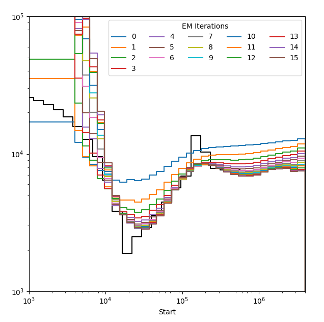
Estimated population size over 15 EM iterations each plotted in a different colour. The model appears to have well converged to a solution.
Plotting migration and effective population size can be done similarly with smcsmc.plot_migration and smcsmc.plot_ne. See the API documentation for more information.