API Documentation
Main Function
smcsmc.run_smcsmc(args)[source]¶The main entry point to
smcsmc, this function runs the whole analysis portion from start to finish. The one single argument is a dictionary of arguments as detailed on the Input Arguments.Tip
It’s a really good idea to run
smcsmcin atmuxsession on the login node of your cluster if you are doing large analyses. The main loop takes very little memory, and spawns off cluster jobs if it is configured to do so (Clustering Computing).
Parameters: args (dict) – A dictionary of arguments as per Input Arguments. An entirely equivalent entry point is the command line interface called
smc2. See Command Line Interface for examples.
smcsmcrequires segment files as input. Below we detail three main ways to create them.
- From VCF files
- From
msprimesufficient tree sequences- From
SCRMsimulationsIf you are using a different data type and would like help converting it to seg format, please let us know. For more details on converting files and interpreting the output of the algorithm, please see Getting Started.
Format Conversions
-
smcsmc.ts_to_seg(path, n=None)[source]¶ Converts a tree sequence into a seg file for use by
smcsmc.run_smcsmcs(). This is especially useful if you are simulating data frommsprimeand would like to directly use it insmcsmc. For details of how to do this, please see the tutorial on simulation usingmsprime.Provide the path to the tree sequence, and the suffix will be replaced by
.seg. This code is adapted from PopSim.Parameters:
-
smcsmc.vcf_to_seg(input, output, masks=None, tmpdir='.tmp', key='tmp', chroms=range(1, 23))[source]¶ This function converts data from a VCF to the segment type required for
smcsmc. You can also (optionally) include masks for the VCF (for example, from 1000 genomes) to indicate callable regions. This function first creates a number of intermediary VCF files intmpdir, identifiable by theirkeyand sample IDs. The function, by default, will loop over all chromosomes and create seperateseg.gzfiles for each of them, however you can specify only a subset of chromosomes by providing a list tochroms.It is preferable for VCFs to be phased, but it is by no means necessary. Phasing helps to improve the effectiveness of the lookahead likelihood.
Warning
This function does not take a lot of memory, but it can run for quite a while with genome-scale VCFs.
The format of the input argument is as follows:
input = [
    ("path_to_vcf", "sample_ID_1"),
    ("path_to_vcf", "sample_ID_2)
]
For each individual that you would like to include in the segment file, you must specify its identifier and the path to its VCF. This means, in some cases, that you will be repeating the VCF paths. That’s okay. Give the pairing of the VCF path and Sample ID (in that order) as a tuple, and give the list of tuples as the input argument. This is the same order in which individual’s genotypes will appear in the seg file.
Chromosomes
If you have one VCF with many chromsoomes, specify the chromosomes that you want to use in the anlaysis in the
chromoption, as mentioned above. If you have many VCFs for each chromosome, you will have to run this function separately for each, specifying the correct chromsome each time.Masks
Masks are bed files which indicate the callable regions from a VCF file, and may be included. If you do include masks, please make sure to include at least as many masks as individuals.
Example
If you wanted to convert two individuals from two different VCFs, whilst specifying masks, for chromosomes 5,6, and 7:
smcsmc.vcf_to_seg(
    input = [
        ("/path/to/vcf1", "name_of_individual_1"),
        ("/path/to/vcf2", "name_of_individual_2")],
    output = "chrs567.seg.gz",
    masks = [
        "/path/to/mask1.bed.gz",
        "/path/to/mask2.bed.gz"],
    key = "chrs567",
    chroms = [5,6,7]
)
Which would create
chr567.seg.gzin the current working directory.Parameters: - input (list) – List of tuples, where the first element is the path to the VCF file and the second is the individual to be included.
- output (str) – Path to the output segment file. Gzipped if the suffix indicates so.
- masks (list) – List of masks for each of the individuals given in
input. These are positive masks. Masks are given as bed files, optionally gzipped. - tempdir (str) – Directory to write intermediary vcf files. This is not cleaned after runs, so make sure you know where it is! This is to preserve the files for any further conversions.
- key (str) – Unique identifier of this run.
- chroms (list) – Either a list or range of chromosomes codes to use in this particular run.
Todo
It would be good to have a “cleanup = True” option to get rid of the intermediary files. This would be highly inefficient for rerunning but maybe worth it for some people.
Returns: Nothing.
Plotting
-
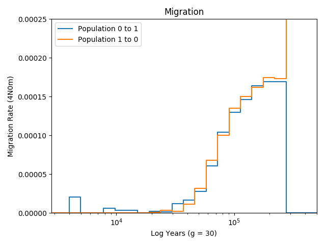
smcsmc.plot.plot_migration(input='result.out', output='result.png', g=30, ymax=0.00025)[source]¶ Plot the migration between two groups.
The function pulls from the input, which must be some sort of aggregated output from
smcsmc, and plots the migration rate over time for a given generational timeg, which scales the number of generations to years. The Y axis (which can be modified with theymaxparameter) represents \(m_{ij}\), or the proportion of population j being placed by migration from population i backwards in time. This is important, as most intution about migration is understood forward in time.This is a barebones function and there is no option to provide a “truth” bar. See the other plotting functions for various definitions of “truth”.
As an example, here is the resulting (symmetric) migration from a simulation:
Todo
Typo above, it is not log years, rather years and the axis is logged.
Parameters: - input (str) – This must be the file path to some sort of aggregated output from
smcsmc. This means that it can be either achunkfinal.outorresult.outbut not an individual chunk. We need all the data here. - output (str) – Filepath to save the plot.
- g (int) – The length of one generation in years. This is used to scale the x axis.
- ymax (float) – The maximum y value to plot. This is used to scale the plots up or down.
- input (str) – This must be the file path to some sort of aggregated output from
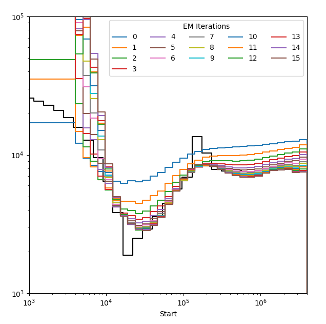
-
smcsmc.plot.plot_rainbow(input, output, g=30, model=None, steps=None, pop_id=1)[source]¶ Creates a plot of all iterations by colour. This plot is useful for assessing convergence.
Parameters: - input (str) – The full file path to an aggregated output file from
smcsmc. - output (str) – Filepath to save the plot.
- g (int) – The length of one generation in years. This is used to scale the x axis.
- model (stdpopsim.Model) – Model for plotting.
- ymax (float) – The maximum y value to plot. This is used to scale the plots up or down.
- steps (int) – Don’t worry about this.
- pop_id (int) – If your model includes multiple populations, which one do you want to plot?
- input (str) – The full file path to an aggregated output file from
-
smcsmc.plot.plot_with_guide(input, guide, output, g=30, ymax=0.00025, N0=14312)[source]¶ This function is very similar to
smcsmc.plot.plot_migration()except that it includes the ability to add a bar of “truth”. In this case, the function uses a specific form of “truth” generated from recording all epochs output bySCRM. Additionally, we provide both the effective population size and the migration rates.The structure of the truth guide is like so:
Start Time Pop_1 Ne Pop_2 Ne Pop_1 M Pop_2 M 0 3 3 6 2 100 0.65 0.3 14 0 … . . . . 10000 0.4 0.4 8 6 Saved as a CSV file for the
guideargument.Todo
This function is part of a WIP tutorial on simulating with
SCRM. More details and convenience functions to come.Parameters: - input (str) – The full file path to an aggregated output file from
smcsmc. - guide (str) – The full file path to a CSV formated as above with the truth of a simulation.
- output (str) – Filepath to save the plot.
- g (int) – The length of one generation in years. This is used to scale the x axis.
- ymax (float) – The maximum y value to plot. This is used to scale the plots up or down.
- input (str) – The full file path to an aggregated output file from