Simulated Data with msprime
Another popular framework for coalescent simulation is msprime, a reimplimentation of Hudson’s ms. In this tutorial we show how to simulate data with msprime under any model and reinfer demographic parmeters with smcsmc.
Data Generation
This is not a guide for using msprime, and if you are unfamiliar with syntax, the documentation is very helpful. Here we are essentially following the analysis implemented in the PopSim analysis comparing multiple tools for demographic inference.
import msprime
from stdpopsim import homo_sapiens

# Here we use a three-population Out of Africa (OoA) model of human history.
#
# It is stored in the stdpopsim homo_sapiens class.
#
# Your model could be anything.
model = getattr(stdpopsim.homo_sapiens, "GutenkunstThreePopOutOfAfrica")

# We are interested in four individuals from the second (European) population.
#
# We take these samples in the present day.
samples = [msprime.Sample(population = 1, time = 0)] * 4

# Perform the simulation
# We pass all of the demographic events from the model as a dictionary to the simulation function.
ts = msprime.simulate(
        samples = samples,
        mutation_rate = 1.25e-8,
        **model.asdict())

# And spit out the tree file.
ts.dump('msprime.tree')
We include functions to convert from tree sequence dumps to the seg files necessary for smcsmc analysis.
import smcsmc

smcsmc.ts_to_seg('msprime.tree')
Which will write msprime.seg in the current working directory. We now, fairly straightforwardly, analysing this seg data using the same procedure outlined in Getting Started.
import smcsmc

args = {
        'EM':                           '15',
        'Np':                           '10000',

        # Submission Parameters
        'chunks':                       '100',
        'c':                            '',
        'no_infer_recomb':              '',

        # Other inference parameters
        'mu':                           '1.25e-9',
        'N0':                           '14312',
        'rho':                          '3e-9',
        'calibrate_lag':                '1.0',
        'tmax':                         '3.5',
        'alpha':                        '0',
        'apf':                          '2',
        'P':                            '133 133016 31*1',
        'VB':                           '',
        'nsam':                         '4',

        # Files
        'o':                            'run',
        'seg':                          'msprime.seg'
}

smcsmc.run_smcsmc(args)
Which creates the following output result.out:
Iter  Epoch       Start         End   Type   From     To            Opp          Count           Rate             Ne         ESS  Clump
15      0           0         133   Coal      0     -1      1646116.6       21.30762  1.2944174e-05      38627.416      1.3013     -1
15      1         133       166.2   Coal      0     -1      872269.46      26.817873  3.0744941e-05      16262.838      1.9003     -1
15      2       166.2      207.68   Coal      0     -1      1357402.8      2.1042327  1.5501903e-06      322541.04      2.1558     -1
15      3      207.68      259.53   Coal      0     -1      2109009.6      14.543791  6.8960285e-06      72505.501      2.4425     -1
15      4      259.53      324.31   Coal      0     -1      3278185.9      49.605303  1.5131937e-05      33042.696      2.7563     -1
15      5      324.31      405.26   Coal      0     -1      5071446.2         172.38  3.3990305e-05      14710.077      3.7783     -1
15      6      405.26      506.42   Coal      0     -1      7753527.6         378.89   4.886679e-05      10231.898       3.719     -1
15      7      506.42      632.82   Coal      0     -1       11654873        1049.43  9.0042165e-05       5552.954      4.6282     -1
15      8      632.82      790.79   Coal      0     -1       16851889        2312.22  0.00013720836      3644.0929      5.2067     -1
15      9      790.79      988.18   Coal      0     -1       23398842        3743.37  0.00015998099      3125.3713      6.1686     -1
15     10      988.18      1234.8   Coal      0     -1       31119159        5716.96   0.0001837119      2721.6527      7.2951     -1
15     11      1234.8      1543.1   Coal      0     -1       40005064        7390.63  0.00018474236      2706.4718      7.5514     -1
15     12      1543.1      1928.2   Coal      0     -1       50983716        8280.42  0.00016241303      3078.5707      9.1861     -1
15     13      1928.2      2409.6   Coal      0     -1       65470637        9105.62  0.00013907945      3595.0675      9.8557     -1
15     14      2409.6        3011   Coal      0     -1       85565757        9585.52  0.00011202519       4463.282      11.876     -1
15     15        3011      3762.6   Coal      0     -1  1.1401707e+08       10315.08  9.0469615e-05      5526.7174      15.182     -1
15     16      3762.6      4701.8   Coal      0     -1  1.5524053e+08       10862.25  6.9970451e-05      7145.8736      17.483     -1
15     17      4701.8      5875.5   Coal      0     -1  2.1375026e+08       12649.97  5.9181073e-05       8448.647       20.76     -1
15     18      5875.5      7342.1   Coal      0     -1  2.9163573e+08       16020.13  5.4931986e-05      9102.1649       27.88     -1
15     19      7342.1      9174.7   Coal      0     -1   3.863795e+08       21177.96  5.4811293e-05      9122.2078      34.639     -1
15     20      9174.7       11465   Coal      0     -1    4.88984e+08       28276.39  5.7826821e-05      8646.5068      43.304     -1
15     21       11465       14327   Coal      0     -1  5.8197353e+08       36240.01  6.2270891e-05      8029.4339      51.301     -1
15     22       14327       17903   Coal      0     -1   6.451339e+08       43546.96  6.7500653e-05      7407.3357      60.539     -1
15     23       17903       22372   Coal      0     -1  6.6748478e+08       47326.54  7.0902801e-05      7051.9076      68.849     -1
15     24       22372       27956   Coal      0     -1  6.4691201e+08       46774.72  7.2304609e-05      6915.1885      74.323     -1
15     25       27956       34934   Coal      0     -1  5.8593471e+08       42400.23  7.2363404e-05      6909.5699      85.549     -1
15     26       34934       43654   Coal      0     -1  4.8670448e+08       34939.75  7.1788428e-05      6964.9108      87.582     -1
15     27       43654       54551   Coal      0     -1  3.6252162e+08       25596.63  7.0607181e-05      7081.4327      93.198     -1
15     28       54551       68167   Coal      0     -1  2.3434808e+08       16196.81  6.9114327e-05        7234.39      76.176     -1
15     29       68167       85183   Coal      0     -1  1.2699601e+08        8639.48  6.8029541e-05      7349.7482      72.283     -1
15     30       85183  1.0645e+05   Coal      0     -1       54744833        3688.46  6.7375491e-05      7421.0962      66.976     -1
15     31  1.0645e+05  1.3302e+05   Coal      0     -1       17948123        1184.46  6.5993531e-05      7576.5002      65.159     -1
15     32  1.3302e+05       1e+99   Coal      0     -1      4926174.5         316.93  6.4335926e-05      7771.7076      72.307     -1
15     -1           0       1e+99  Delay     -1     -1  3.0934923e+09              0              0              0           1     -1
15     -1           0       1e+99 Recomb     -1     -1           3300  9.9000003e-06  3.0000001e-09              0           1     -1
15     -1           0       1e+99 Resamp     -1     -1  3.0934923e+09         882448  0.00028525948              0           1     -1
Of course your output will not be the same, but if you have properly set up smcsmc to use a compute cluster and given it sufficient time to execute, then the resulting trends will be highly similar.
Todo
Combine the functions to produce a plot with a guide so that I can show it here. Currently I have a SCRM plot with guide and an msprime plot from stdpopsim but not both.
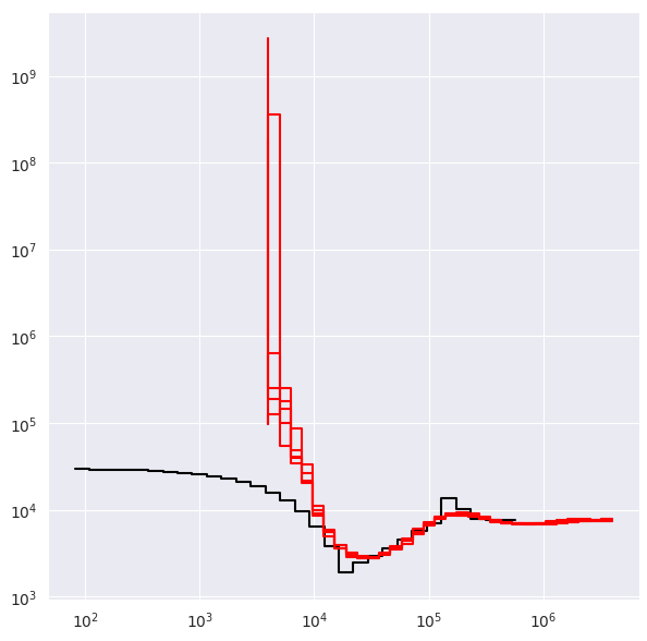
Five replications of this leads to the following results: